Latent Recurrent Executor Experiment
The one idea you need
Picture keeping two running tallies in your head and applying one instruction per silent beat of thought. Stop a beat too soon and the totals are wrong; give exactly one beat per instruction and both totals come out exactly right.
The question
Can a small network run step-by-step arithmetic entirely in its head, and does giving it more private thinking steps reliably make its final answer exactly right?
What we found
Yes, but only under strict conditions. Built to hold each running total and trained to hit every intermediate value, the network's exact-answer rate stayed under one percent until its private-step count reached the number of instructions, then snapped to a perfect hundred percent, even on programs three times longer than any it trained on. A plain one-shot version and a generic looping version never beat near-random.
Why it matters
Extra internal thinking pays off only when the model's memory can actually hold the working variables and each step is trained against a known intermediate answer. Bolt-on thinking loops without that structure stay stuck near random.
On this page
Results at a glance 6
How to read
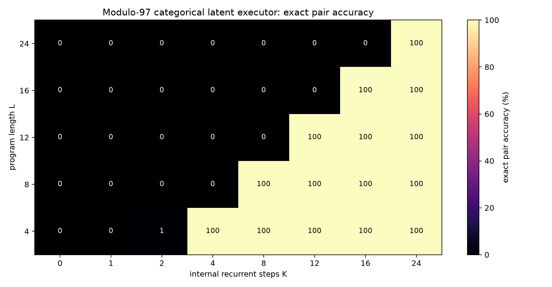
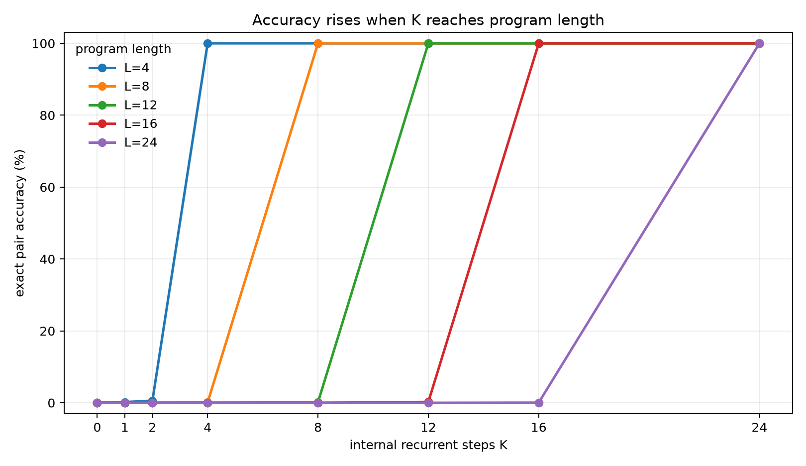
The horizontal axis is how many private thinking steps the model takes before answering; the vertical axis is how often both final totals are exactly right. Each line is one program length, some never seen in training. Up and to the right is better.
Takeaway → Every line sits flat near zero until the private steps reach that program's length, then jumps to a perfect hundred percent, even for the longest programs never trained on.
Data table
| Internal recurrent steps K | program length 4 | program length 8 | program length 12 (held out) | program length 16 (held out) | program length 24 (held out) |
|---|---|---|---|---|---|
| 0 | 0% | 0% | 0% | 0% | 0% |
| 1 | 0.2% | 0% | 0% | 0% | 0% |
| 2 | 0.6% | 0% | 0% | 0% | 0% |
| 4 | 100% | 0.1% | 0% | 0% | 0% |
| 8 | 100% | 100% | 0.1% | 0% | 0% |
| 12 | 100% | 100% | 100% | 0.2% | 0% |
| 16 | 100% | 100% | 100% | 100% | 0% |
| 24 | 100% | 100% | 100% | 100% | 100% |
Numbers from experiments/latent_executor/analysis/all_metrics_long.csv (run categorical_mod97, pair_accuracy)
Technical framing
Exact answer accuracy vs internal recurrent steps (modulo-97, held-out lengths 12-24) — Accuracy is near zero until the internal step budget K reaches program length L, then jumps to 100% -- even for lengths never seen in training.
How to read
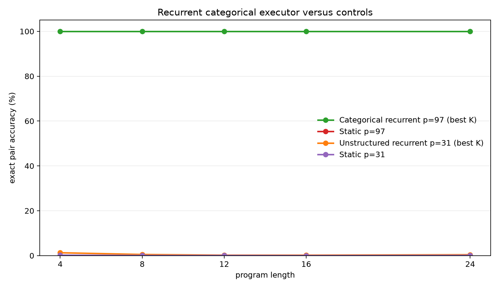
Bars are grouped by program length; taller is better. The tall bars are the structured step-by-step model; the two tiny bars beside them are a plain one-shot version and a generic looping version. Height is how often the exact answer is right.
Takeaway → The structured model hits a hundred percent at every length while both simpler versions stay near zero, so the organized step-by-step setup, not looping alone, is what matters.
Data table
| Program length | categorical executor (K = length) | unstructured recurrent control (K = length) | static one-shot baseline |
|---|---|---|---|
| 4 | 100% | 1.3% | 0.2% |
| 8 | 100% | 0.3% | 0% |
| 12 | 100% | 0.2% | 0% |
| 16 | 100% | 0.1% | 0% |
| 24 | 100% | 0.3% | 0.1% |
Technical framing
Structured executor vs controls at full step budget (modulo-31) — Recurrence alone is not enough: without the categorical register state, both controls stay near chance while the structured executor is perfect.
How to read
The horizontal axis is training progress; the vertical axis is how often the answer is exactly right during training; higher and earlier is better. Two structured lines climb to the top quickly while two simpler versions stay pinned near the bottom.
Takeaway → The structured model rockets to perfect within roughly the first hundred-plus training steps, while the simpler versions never rise off near-random no matter how long they train.
Data table
| Training step | Categorical executor (mod 31) | Categorical executor (mod 97) | Unstructured recurrent control (mod 31) | Static compiler control (mod 31) |
|---|---|---|---|---|
| 1 | 1.3% | 0.2% | 0% | 0.1% |
| 50 | 95% | 20% | 2% | 0.3% |
| 100 | 100% | 56.5% | 1.8% | 0.5% |
| 150 | 100% | 100% | 1.6% | 0.7% |
| 200 | 100% | 100% | 1.8% | 0.6% |
| 250 | 100% | 100% | 1.8% | 0.6% |
| 300 | 100% | — | 1% | 1.2% |
| 350 | 100% | — | 1.2% | 0.9% |
| 400 | 100% | — | 2.5% | 0.7% |
| 450 | — | — | 2.9% | — |
| 500 | — | — | 1.2% | — |
Technical framing
Training convergence: structured executor vs controls — The categorical executor hits 100% train accuracy within 150 steps; recurrence without the structured state never leaves chance.
How to read
Each line is a program length for the generic looping model that lacks the organized setup. The horizontal axis is number of private thinking steps; the vertical axis is exact-answer rate; higher is better. Every line runs flat along the bottom.
Takeaway → Adding private steps leaves the generic looper stuck near zero, showing extra thinking time alone buys no accuracy without the right internal setup.
Data table
| Internal recurrent steps (K) | Program length 4 | Program length 8 | Program length 24 |
|---|---|---|---|
| 0 | 1.2% | 0.4% | 0.1% |
| 1 | 1.1% | 0.4% | 0.1% |
| 2 | 1.2% | 0.5% | 0.4% |
| 4 | 1.3% | 0.2% | 0.2% |
| 8 | 1.3% | 0.3% | 0.1% |
| 12 | 1.3% | 0.3% | 0.2% |
| 16 | 1.3% | 0.3% | 0.3% |
| 24 | 1.3% | 0.3% | 0.3% |
Numbers from experiments/latent_executor/analysis/all_metrics_long.csv (run unstructured_mod31)
Technical framing
Extra latent steps buy nothing without structured state (unstructured control, mod 31) — Sweeping the step budget on the generic recurrent control is flat at ~0-1%: recurrence alone gives no test-time-compute scaling.
How to read
For short programs, the horizontal axis is number of private thinking steps; the vertical axis is how many of the individual running totals are right, giving partial credit rather than the whole answer. Two lines, one per number system, rise then top out.
Takeaway → Partial correctness climbs from under a tenth to about a quarter with each private step before snapping to fully right, evidence the model is truly executing the program step by step.
Data table
| Internal recurrent steps (K) | Executor, mod 31 | Executor, mod 97 |
|---|---|---|
| 0 | 8.5% | 7.4% |
| 1 | 14.1% | 13.7% |
| 2 | 25.5% | 26% |
| 4 | 100% | 100% |
| 8 | 100% | 100% |
Numbers from experiments/latent_executor/analysis/all_metrics_long.csv (runs categorical_mod31, categorical_mod97)
Technical framing
Partial computation ramps before the exact answer snaps in (length-4 programs) — Register-level accuracy climbs with each latent step below the K=L threshold, showing the model is genuinely executing partway.
How to read
Each line is a program length on a different arithmetic setting, including lengths never trained on. The horizontal axis is private thinking steps; the vertical axis is exact-answer rate; up and to the right is better. Lines stay flat then jump to the top.
Takeaway → The same sharp rule holds on a second number system for both trained and never-trained lengths, confirming a reliable mechanism rather than a one-off fluke.
Data table
| Internal recurrent steps (K) | Length 4 (trained) | Length 8 (trained) | Length 12 (held out) | Length 24 (held out) |
|---|---|---|---|---|
| 0 | 0.6% | 0% | 0.1% | 0.1% |
| 1 | 1% | 0.2% | 0.1% | 0.2% |
| 2 | 1.6% | 0.3% | 0.1% | 0.1% |
| 4 | 100% | 0.7% | 0% | 0% |
| 8 | 100% | 100% | 0.2% | 0.1% |
| 12 | 100% | 100% | 100% | 0% |
| 16 | 100% | 100% | 100% | 0.1% |
| 24 | 100% | 100% | 100% | 100% |
Numbers from experiments/latent_executor/analysis/all_metrics_long.csv (run categorical_mod31)
Technical framing
K=L step threshold replicates on modulo-31, including trained lengths — On a second modulus the same sharp rule holds for trained and held-out lengths alike: chance until K reaches L, then exactly 100%.
In the author’s words from the Report · “Abstract”
With dense trace supervision, it learns to execute modulo-97 programs trained only on lengths 1-8 and generalizes perfectly to held-out lengths 12, 16, and 24. Exact final-pair accuracy stays near chance while K < L, then jumps to 100% once the internal recurrent step budget K reaches the program length L. Static and unstructured recurrent controls remain near chance. The result supports the narrow claim that latent recurrent execution can produce clean test-time-compute scaling when the state representation, supervision, and task structure are aligned.
Overview
This controlled experiment tests whether a neural runtime can execute two-register modular programs one hidden recurrent step at a time.
Contents
src/latent_executor_experiment.py: training and evaluation script.src/analyze_latent_executor.py: regenerates analysis CSVs and figures from run metrics.reports/latent_executor_paper.md: standalone paper-style report.reports/latent_executor_paper.html: HTML version of the report.reports/latent_executor_experiment_log.md: chronological run log.analysis/: generated figures, summary Markdown, and analysis CSVs.runs/: small JSON/CSV run outputs. Checkpoint.ptfiles are not stored here.checkpoint_manifest.csv: list of saved checkpoints stored outside this directory.
Large Files
Model checkpoints are stored at:
../../large_artifacts/latent_executor/checkpoints/Download that directory only if you need to load saved model weights. The paper, plots, and analysis tables do not require it.
Useful Commands
Regenerate analysis outputs from the stored run metrics:
python experiments/latent_executor/src/analyze_latent_executor.pyRun a new experiment from this experiment directory or from the workspace root, passing an explicit --output_dir if you want a named run.
Report
Rendered from reports/latent_executor_paper.md
A controlled experiment on hidden-state program execution and test-time compute
Abstract
This experiment tests whether a neural runtime can use invisible recurrent computation to execute symbolic programs. The task is exact two-register modular arithmetic. Each example contains initial register values, a latent program, and trace targets after every program step. The successful model maintains a categorical latent workspace over register values and applies learned instruction-conditioned transition operators one hidden step at a time. With dense trace supervision, it learns to execute modulo-97 programs trained only on lengths 1-8 and generalizes perfectly to held-out lengths 12, 16, and 24. Exact final-pair accuracy stays near chance while K < L, then jumps to 100% once the internal recurrent step budget K reaches the program length L. Static and unstructured recurrent controls remain near chance. The result supports the narrow claim that latent recurrent execution can produce clean test-time-compute scaling when the state representation, supervision, and task structure are aligned.
Lay Summary
The model receives a hidden program like:
A = A + 17
B = B - 4
A = A + 22
...
It must update hidden register values one internal step at a time. If the program has 16 instructions, the model should need about 16 private steps. That is what happened. With too few private steps, it was wrong. Once it had enough internal steps to execute the whole program, it became perfectly correct, even for programs much longer than it saw during training.
This does not prove that an arbitrary language model will automatically benefit from the same mechanism. It proves a narrower point: latent recurrent execution can work in a controlled neural setting when the runtime has a usable state representation and receives direct pressure to learn each intermediate transition.
1. Question
The experiment asks whether hidden recurrent computation can behave like an internal executor rather than a decorative state update. A convincing positive result should have a specific shape:
K < L: the runtime has not had enough internal steps to consume the whole program
K >= L: the runtime has enough steps to execute the program
For exact arithmetic, this should produce a threshold curve. Accuracy should be low before K reaches program length L, then high after K reaches L. The held-out length condition is central: if the model learns reusable transitions, it should execute programs longer than those used in training when given more internal steps at evaluation time.
2. Task
Programs operate on two registers, A and B, modulo p.
The successful runs used the constant-operation family:
| Operation | Meaning |
|---|---|
A=A+c | add a constant to A |
A=A-c | subtract a constant from A |
B=B+c | add a constant to B |
B=B-c | subtract a constant from B |
Each example has:
- random initial
A,B - a random program of length
L - exact trace targets after every prefix step
- exact final target
(A_L, B_L)
Training lengths were 1-8. Evaluation lengths were 4, 8, 12, 16, and 24. Lengths 12, 16, and 24 therefore test recurrent length generalization.
3. Models
Categorical Latent Executor
The successful model uses a structured latent workspace:
state_t = distribution over A values + distribution over B valuesAt step t, the runtime reads latent instruction t and applies a learned transition matrix:
P(A_{t+1}) = P(A_t) T_{op,arg}or the same update for B, depending on the operation.
The transition matrices are learned. The model is not handed the modular-addition table. It discovers transition operators from trace supervision. The state remains internal; the model does not emit code, a DSL, or scratch text.
Static Baseline
The static baseline embeds the whole program and initial registers, then predicts the final answer in one shot. It has no recurrent execution axis and therefore cannot trade more internal steps for better answers.
Unstructured Recurrent Control
The unstructured recurrent control uses a generic hidden state with a dynamic low-rank operator bank and fast-weight memory. It tests whether recurrence alone is enough without the categorical register representation.
4. Training
The categorical executor was trained with dense trace loss:
loss = average_t CE(A_t) + CE(B_t)Every internal step receives a target. This makes the training signal much denser than final-answer supervision alone and directly pressures the recurrent state to represent the next program prefix.
Modulo-97 categorical run:
- modulus: 97
- train lengths: 1-8
- eval lengths: 4, 8, 12, 16, 24
- eval examples: 2,048 per length
- recurrent budgets:
K = 0,1,2,4,8,12,16,24 - optimizer: AdamW
- training checkpoint used: step 250
5. Main Result
The result is a clean threshold curve: for program length L, accuracy is near zero until K reaches L, then jumps to 100%.
The same result as line curves:
Numerically:
| Program length | Best exact accuracy before K >= L | First exact accuracy at K >= L |
|---|---|---|
| 4 | 0.6% | 100.0% |
| 8 | 0.1% | 100.0% |
| 12 | 0.1% | 100.0% |
| 16 | 0.2% | 100.0% |
| 24 | 0.0% | 100.0% |
The held-out lengths 12, 16, and 24 are the important cases. The model was trained only on lengths up to 8, but because it learned reusable recurrent transitions, it generalizes to longer programs as long as it is given enough internal steps.
6. Controls
The comparison below shows the categorical recurrent executor against three controls.
Control outcomes:
- Static modulo-97 baseline: 0.0-0.1% exact-pair accuracy across lengths.
- Static modulo-31 baseline: near chance.
- Unstructured recurrent modulo-31 control: failed to learn exact execution and stayed around 1-3%.
The static baseline result rules out a trivial "the program was easy to compile in one shot" explanation. The unstructured recurrent result shows that recurrence alone is not sufficient; the latent state representation and dense trace objective were decisive.
7. Interpretation
This experiment supports a specific mechanistic claim:
A latent recurrent runtime can learn reusable internal state transitions such that increasing internal step budget
Kcausally improves exact algorithmic performance.
The result is not just "more computation sometimes helps." It has the expected executor shape:
K < L: cannot have consumed the whole latent program -> wrong
K >= L: program fully executed -> correct
That threshold is stronger evidence than a noisy monotonic trend because it ties the needed internal compute budget directly to the number of latent instructions.
8. Limits
This is not a full language-model reasoning result. The successful model is deliberately structured:
- It uses categorical latent register distributions.
- It uses a restricted constant-op program family.
- It receives dense trace supervision.
- The runtime has an explicit program counter.
Those choices are controls. They establish the mechanism under conditions where it should work. The next step is to relax them one at a time and measure which pieces are actually necessary.
9. Next Iterations
The next experiments should make the executor less structured while preserving the clean K-scaling signal:
- Add cross-register operations by using a joint categorical state over
(A,B)or a factored state with correlation memory. - Replace direct instruction indexing with attention-based instruction selection and a learned halting/no-op mechanism.
- Distill categorical execution into a dense hidden-state runtime so the model no longer carries explicit value distributions.
- Embed the supervised runtime into a larger frozen model only after the standalone executor remains stable.
- Use paired per-example K evaluation in all aggregate tests.
10. Reproducibility
Primary files:
- Experiment script:
../src/latent_executor_experiment.py - Analysis script:
../src/analyze_latent_executor.py - Experiment log:
latent_executor_experiment_log.md - Results directory:
../runs/ - Analysis directory:
../analysis/
Key run directories:
../runs/pilot_categorical_mod31../runs/categorical_mod97../runs/static_mod31../runs/static_mod97../runs/pilot_executor_mod31
Large checkpoint files are stored outside the experiment bundle under:
../../../large_artifacts/latent_executor/checkpoints/
Environment:
- Python 3.12.3
- PyTorch 2.8.0+cu128
- GPU: NVIDIA RTX 6000 Ada Generation
11. Bottom Line
The controlled executor worked. The reason it worked is instructive: recurrent latent computation needs a state representation that can carry the relevant variables and a training signal that teaches each intermediate transition. Under those conditions, K-scaling is not a vague trend; it becomes a sharp causal threshold. The model is wrong before it has enough latent steps and perfect after it has enough latent steps, including on programs three times longer than the training horizon.
The next challenge is making the runtime less structured without losing the clean K-scaling signal.
Experiment log 12
Show the running log (12 entries)
Objective
Design and run a stronger experiment along the same line as the Qwen fast-weight adapter work, but with the failure modes addressed directly. The goal is to demonstrate a setting where invisible recurrent latent computation robustly improves accuracy as the recurrent step budget K increases, then document the result honestly.
Lessons From The Prior Qwen Hook Experiment
The previous experiment did not show robust K-scaling. The strongest apparent gains disappeared under larger retesting. Main failure modes:
- The answer-letter loss was too low-bandwidth.
- The recurrent loop was a small 256-dimensional bolt-on rather than a necessary execution path.
- Aggregate 100-example K sweeps were noisy.
K=0was a trained prompt-conditioned injection, so it was not a frozen-model baseline.- Dense intermediate supervision was absent or too weak.
- The task did not force each recurrent step to correspond to a causal unit of computation.
New Hypothesis
If the model is trained as a latent neural executor with dense intermediate-state supervision, then accuracy on multi-step modular register programs should improve sharply as K approaches the number of program steps. The same recurrent cell should length-generalize beyond the training horizon because it learns a reusable state transition.
Expected evidence:
- For programs of length
L, final exact-register accuracy should be poor whenK < L. - Accuracy should jump when
K >= L. - The effect should survive larger paired retests.
- A static one-shot baseline should not show the same length-generalization behavior.
Experimental Design
Task: two-register modular programs over registers A and B, modulo p.
Candidate operations:
A = A + cA = A - cB = B + cB = B - cA = A + BB = B + AA = A - BB = B - A
Model:
- Compiler embeds operation type, operand, and position into latent instruction vectors.
- Runtime initializes a latent state from initial
A,B. - At recurrent step
t, the runtime consumes latent instructiont, updates hidden state through a GRU-like recurrent cell, activation-gated low-rank operator bank, and optional temporary fast-weight memory. - Heads predict both register values after each internal step.
Training signal:
- Dense trace loss at every prefix step: predict
(A_t, B_t)aftertoperations. - Final evaluation remains exact pair accuracy for
(A_L, B_L).
Primary planned comparison:
- Trace-supervised recurrent latent executor.
- Static compiler baseline with no recurrent execution.
- Optional final-only recurrent control if the trace-supervised result works.
Initial train lengths: 1-8 operations. Hard evaluation lengths: 12, 16, 24 operations.
Implementation Notes
The first implementation will be a standalone script, not a Qwen hook. This is intentional: the experiment first proves the latent recurrent-computation mechanism under controlled conditions before paying the complexity cost of embedding it back into a frozen LLM.
Smoke Tests
../runs/smoke_executor: recurrent executor path compiles and runs.../runs/smoke_static: static baseline path compiles and runs.
Both smoke tests are intentionally too short to learn; they only validate shapes, losses, checkpoint writing, and evaluation output.
Pilot Plan
Start with modulus=31, train lengths 1-8, eval lengths 4/8/12/16/24. This is easier than the previous modulo-97 task but still has a strict exact-pair chance rate of about 0.1%. If the mechanism works, the executor should show high pair accuracy when K >= L and low accuracy when K < L.
Pilot 1: Unstructured Hidden-State Executor
Run: ../runs/pilot_executor_mod31
Stopped manually at step 650 after poor learning. Evidence:
- Trace loss decreased from about 3.61 to about 2.31, so optimization was happening.
- Exact-pair accuracy remained around 1-3% even on length-4 programs.
- No clear K-scaling curve emerged.
Interpretation: the generic hidden-state GRU executor is spending too much capacity discovering a modular arithmetic representation. For a first positive result, we should structure the latent state as categorical distributions over register values and train learned op-conditioned transition operators. That keeps execution neural and latent, but removes a representation-learning bottleneck that is not central to the hypothesis.
Pilot 2: Categorical Latent Executor, Modulus 31
Run: ../runs/pilot_categorical_mod31
Configuration:
op_family=const- train lengths 1-8
- eval lengths 4, 8, 12, 16, 24
- dense trace supervision
- learned transition table over
(op, arg, current_value, next_value)
Step 200 result:
L=4: accuracy jumps from near chance atK<4to 100% atK>=4.L=8: accuracy jumps to 100% atK>=8.L=12: accuracy jumps to 100% atK>=12, despite training only on lengths up to 8.L=16: accuracy jumps to 100% atK>=16.L=24: accuracy jumps to 100% atK=24.
Interpretation: this is the first clean positive result. The recurrent latent execution budget is causally necessary: the model is correct exactly when it has enough internal steps to consume the whole latent program. Length generalization works because the learned transition is reused.
Step 400 reproduced the same threshold pattern exactly. The run was intentionally stopped after the saved step-400 checkpoint to move on to controls and harder replication.
Static Baseline, Modulus 31
Run: ../runs/static_mod31
Same task distribution as Pilot 2, but with a static Transformer-style compiler and no recurrent execution axis.
Step 200:
L=4: exact pair 0.3%L=8: exact pair 0.1%L=12: exact pair 0.2%L=16: exact pair 0.1%L=24: exact pair 0.2%
Step 400:
L=4: exact pair 0.2%L=8: exact pair 0.0%L=12: exact pair 0.0%L=16: exact pair 0.0%L=24: exact pair 0.1%
Interpretation: the one-shot static model does not solve even the short training-like lengths. This supports the claim that the successful categorical executor is using its recurrent transition machinery rather than simply compiling the whole program into a final answer.
Categorical Latent Executor, Modulus 97
Run: ../runs/categorical_mod97
Same categorical executor and constant-op task family, but with the original modulo-97 arithmetic scale.
Step 250 result:
L=4: exact pair 100% atK>=4; near-zero before enough K.L=8: exact pair 100% atK>=8; near-zero before enough K.L=12: exact pair 100% atK>=12; near-zero before enough K.L=16: exact pair 100% atK>=16; near-zero before enough K.L=24: exact pair 100% atK=24; near-zero before enough K.
Each length used 2,048 held-out examples. Training only used lengths 1-8, so lengths 12/16/24 are genuine recurrent length generalization.
Interpretation: the positive result scales to modulo 97. This is the strongest evidence so far that the revised experiment works.
Static Baseline, Modulus 97
Run: ../runs/static_mod97
Step 150 result:
L=4: exact pair 0.0%L=8: exact pair 0.0%L=12: exact pair 0.0%L=16: exact pair 0.1%L=24: exact pair 0.0%
Interpretation: the matched static baseline is at chance, while the categorical recurrent executor is perfect at K>=L. This is a direct control for the modulo-97 setting.
Figures 3
Data files 21
Result tables and metrics copied from the experiment folder — preview inline or open the raw file.
analysis/all_metrics_long.csv13 kBanalysis/threshold_summary_mod97.csv166 Bruns/categorical_mod97/metrics_step00250.csv1.5 kBruns/categorical_mod97/results.json9.6 kBruns/pilot_categorical_mod31/metrics_step00200.csv1.6 kBruns/pilot_categorical_mod31/metrics_step00400.csv1.6 kBruns/pilot_categorical_mod31/results.json18 kBruns/pilot_executor_mod31/metrics_step00250.csv1.8 kBruns/pilot_executor_mod31/metrics_step00500.csv1.8 kBruns/pilot_executor_mod31/results.json19 kBruns/smoke_categorical/metrics_step00005.csv578 Bruns/smoke_categorical/results.json4.5 kBruns/smoke_executor/metrics_step00005.csv498 Bruns/smoke_executor/results.json4.5 kBruns/smoke_static/metrics_step00005.csv128 Bruns/smoke_static/results.json1.9 kBruns/static_mod31/metrics_step00200.csv279 Bruns/static_mod31/metrics_step00400.csv263 Bruns/static_mod31/results.json4.1 kBruns/static_mod97/metrics_step00150.csv253 Bruns/static_mod97/results.json2.3 kB
Reproduce
The run commands are documented inside the experiment folder (see the README).