Belief Filter Executor Experiment
The one idea you need
Picture a safe with two dials known only to differ by a fixed amount, so many combinations stay possible. Each instruction turns a dial or rules some settings out. The model holds the whole list of still-possible dial pairs and revises it one instruction at a time.
The question
Can a small model hold every possible answer at once and narrow that list down, one instruction at a time, as it works through a program?
What we found
Yes. When the model runs one internal update per instruction, it lands over 91% of its confidence on the exact set of still-possible answers, versus under 14% when it stops before finishing. It even runs programs three times longer than any it trained on, but only when it tracks the two hidden numbers as a linked pair, not separately, which scored under 4%.
Why it matters
For small models doing multi-step stateful logic, give internal thinking steps that scale with the number of steps, and shape memory to capture how variables relate, not each variable in isolation.
On this page
Results at a glance 6
How to read
Grouped bars by program length. Bar height is the share of confidence placed on the correct set of answers; taller is better. One bar is the full step-by-step tracker; two are shortcut methods that skip it.
Takeaway → The full-tracking bars stand near or above 91% at every length while both shortcut bars hug the floor under 6%, so full tracking is essential.
Data table
| Program length | joint recurrent filter | marginal recurrent control | static compiler control |
|---|---|---|---|
| L=4 | 96.2% | 3.9% | 5.4% |
| L=8 | 93.9% | 2.9% | 2.1% |
| L=12 | 92.4% | 2.3% | 0.7% |
| L=16 | 91.7% | 1.7% | 0.3% |
| L=24 | 91.3% | 1.4% | 0.2% |
Numbers from experiments/belief_filter_executor/analysis/mod31_control_summary.csv
Technical framing
Joint belief state vs controls: probability mass on correct states (mod 31) — Only the joint recurrent filter exceeds 91% target mass at every length; both controls stay under 6%, so joint state and recurrence both matter.
How to read
Each line is one program length. The horizontal axis is how many internal steps the model takes; vertical is confidence on the correct answers, higher is better. Watch where each line leaps upward.
Takeaway → Every line stays near zero then jumps above 91% exactly when the step count reaches that program's instruction count, even for lengths never trained on.
Data table
| Internal recurrent steps K | L=4 | L=8 | L=12 (held-out) | L=16 (held-out) | L=24 (held-out) |
|---|---|---|---|---|---|
| 0 | 2% | 0.9% | 0.6% | 0.3% | 0.2% |
| 1 | 6.9% | 1.3% | 0.4% | 0.4% | 0.2% |
| 2 | 13.8% | 1.9% | 0.5% | 0.4% | 0.1% |
| 4 | 96.2% | 3.8% | 0.6% | 0.4% | 0.3% |
| 8 | 96.2% | 93.9% | 3.1% | 0.5% | 0.2% |
| 12 | 96.2% | 93.9% | 92.4% | 2.6% | 0.1% |
| 16 | 96.2% | 93.9% | 92.4% | 91.7% | 0.8% |
| 24 | 96.2% | 93.9% | 92.4% | 91.7% | 91.3% |
Numbers from experiments/belief_filter_executor/analysis/final_metrics_long.csv (run main_joint_mod31, step 500)
Technical framing
Execution threshold: target mass jumps once step budget K reaches program length L — Mass stays under 14% while K<L and jumps above 91% exactly when K>=L, even at lengths 12-24 the model never saw in training (lengths 1-8).
How to read
Two bars per program length: best confidence when the model has too few steps, versus confidence once it takes one step per instruction. Taller is better.
Takeaway → The too-few-steps bar stays under 14% and the one-step-per-instruction bar jumps over 91%, so the flip happens right at that boundary.
Data table
| Program length | best with K<L | at first K>=L |
|---|---|---|
| L=4 | 13.8% | 96.2% |
| L=8 | 3.8% | 93.9% |
| L=12 | 3.1% | 92.4% |
| L=16 | 2.6% | 91.7% |
| L=24 | 0.8% | 91.3% |
Numbers from experiments/belief_filter_executor/analysis/mod31_threshold_summary.csv
Technical framing
Before vs at the threshold: best mass with too few steps vs mass at K=L — One extra step at the K=L boundary takes target mass from under 14% to over 91%; top-1-on-support hits 100% at the same point.
How to read
Two bars per program length compare an earlier training checkpoint against the final one, both scored at one step per instruction. Height is confidence on the correct answers; taller is better.
Takeaway → The final bars are higher at every length, with the biggest gain on the longest programs, so extra training mainly sharpens an ability that already worked.
Data table
| Program length L (evaluated at K = L) | Step 250 | Step 500 |
|---|---|---|
| L=4 | 88% | 96.2% |
| L=8 | 80.6% | 93.9% |
| L=12 | 77.2% | 92.4% |
| L=16 | 74.8% | 91.7% |
| L=24 | 74% | 91.3% |
Technical framing
Mid-training vs final: extra training tightens the belief state at every length — The K=L threshold already exists at step 250; steps 250-500 mostly sharpen mass, with the biggest gain (+17pp) at the longest programs.
How to read
Grouped bars by program length in a smaller version of the task. Height is confidence on the correct answers; taller is better. Bars compare the full tracker against two shortcut methods.
Takeaway → The full tracker again holds 92-96% while both shortcut methods stay under 18%, so the advantage does not depend on the problem's size.
Data table
| Program length L (evaluated at K = L) | Joint recurrent p=11 | Marginal recurrent p=11 | Static p=11 |
|---|---|---|---|
| L=3 | 96.2% | 10.7% | 17.5% |
| L=6 | 94.1% | 10.2% | 8.2% |
| L=9 | 93% | 8.9% | 3.4% |
| L=12 | 92.2% | 7.9% | 2.3% |
Numbers from experiments/belief_filter_executor/analysis/summary.md (Final Metrics By Run table)
Technical framing
Mod-11 pilot replicates the result: joint beats marginal and static controls — The joint-vs-controls gap is not modulus-specific: at p=11 the joint model holds 92-96% mass while both controls stay under 18%.
How to read
Two falling lines against program length. One line is the average count of answers still possible; the other is how surprised the model is by the true answer. Lower means fewer possibilities and a closer answer.
Takeaway → Both lines fall as programs lengthen, because each added filter shrinks the possibilities from about 13 down to under 2, making the final answer easier to pin down.
Data table
| Program length L | Mean support size (states consistent with observations) | Target NLL |
|---|---|---|
| 4 | 13.1 | 2.2 |
| 8 | 6.47 | 1.5 |
| 12 | 4.17 | 1.08 |
| 16 | 2.75 | 0.785 |
| 24 | 1.7 | 0.441 |
Numbers from experiments/belief_filter_executor/analysis/summary.md (Main Modulus-31 Threshold Summary)
Technical framing
Why longer programs look easier: filtering shrinks the feasible state set — More observations collapse the support from 13 states to 1.7, so target NLL falls with length even though execution is longer.
In the author’s words from the Report · “Abstract”
A program then applies arithmetic updates and observation filters such as A % m = r or B % m = r. The target is the exact final probability distribution over all (A,B) pairs. The primary model stores a joint categorical belief over all register pairs and applies one learned update per internal recurrent step. On the scaled modulus-31 task, it was trained on program lengths 1-8 and evaluated on lengths 4, 8, 12, 16, and 24. Target-support mass stayed low when the internal step budget K was below program length L, then rose above 91% once K>=L. Top-1-on-support reached 100% at the same threshold for every evaluated length. … Read the full result →
Overview
This experiment tests latent recurrent execution over correlated belief states with both arithmetic transitions and observation/filter operations.
Contents
src/belief_filter_executor_experiment.py: training and evaluation harness.src/analyze_belief_filter_executor.py: analysis and figure generation.reports/belief_filter_executor_paper.md: standalone writeup.reports/belief_filter_executor_paper.html: standalone HTML report.reports/belief_filter_executor_experiment_log.md: chronological experiment log.runs/: JSON and CSV run outputs.analysis/: generated summaries and figures.checkpoint_manifest.csv: paths and sizes for saved checkpoints.
Checkpoints are written outside the experiment directory under:
../../large_artifacts/belief_filter_executor/checkpoints/Download this experiment directory for the normal research bundle. Download ../../large_artifacts/belief_filter_executor/ only when saved model weights are needed.
Report
Rendered from reports/belief_filter_executor_paper.md
A controlled experiment on hidden-state execution with arithmetic updates and observations
Abstract
This experiment tests whether a latent recurrent runtime can maintain and update a correlated belief state. Each example starts with an unknown pair of modular registers constrained by B=A+d (mod p). A program then applies arithmetic updates and observation filters such as A % m = r or B % m = r. The target is the exact final probability distribution over all (A,B) pairs.
The primary model stores a joint categorical belief over all register pairs and applies one learned update per internal recurrent step. On the scaled modulus-31 task, it was trained on program lengths 1-8 and evaluated on lengths 4, 8, 12, 16, and 24. Target-support mass stayed low when the internal step budget K was below program length L, then rose above 91% once K>=L. Top-1-on-support reached 100% at the same threshold for every evaluated length. A marginal recurrent control and a static one-shot compiler failed on the scaled task, showing that both joint state and recurrent execution are doing useful work.
Lay Summary
The model begins with partial knowledge:
B = A + d (mod p)This relation describes many possible starting worlds. The program then changes the registers and sometimes adds observations:
A = A + 7
B = B - A
observe A % 5 = 2
A = A + B
The correct answer is not one value. It is the set of all (A,B) pairs still possible after executing the program and filtering by the observations. The joint recurrent model learns to update that whole belief state one instruction at a time. If a program has 16 instructions, it needs 16 internal steps; with fewer steps it has not executed the whole program.
1. Question
The experiment asks whether a learned recurrent runtime can execute belief-state programs when the hidden state must preserve correlations between variables.
The desired evidence has four parts:
- Accuracy should depend on the internal recurrent step budget
K. - The threshold should align with program length
L: weak whenK<L, strong whenK>=L. - Lengths beyond the training range should work when enough recurrent steps are available.
- Controls without joint state or without recurrent execution should fail.
The setting is intentionally controlled. The point is not to test open-ended language reasoning; it is to isolate whether recurrent latent execution can implement exact filtering over a known state space.
2. Task
Programs operate over two registers modulo p.
Initial belief:
{(A, B): B = A + d mod p}For p=31, the full state space has 31 * 31 = 961 register pairs, and the initial support contains 31 of them.
Operations:
| Operation | Meaning |
|---|---|
A=A+c | add a constant to A |
A=A-c | subtract a constant from A |
B=B+c | add a constant to B |
B=B-c | subtract a constant from B |
A=A+B | add B into A |
B=B+A | add A into B |
A=A-B | subtract B from A |
B=B-A | subtract A from B |
OBS_A_BUCKET | filter to states where A % m = r |
OBS_B_BUCKET | filter to states where B % m = r |
Observation residues are sampled from the live support, so every target support is non-empty. For the scaled run, p=31, m=5, and each instruction is an observation with probability 0.3.
Each example has:
- a random relation parameter
d - a random program of length
L - exact belief targets after each program prefix
- an exact final target distribution
Training used lengths 1-8. Evaluation used lengths 4, 8, 12, 16, and 24. Lengths 12, 16, and 24 test length generalization.
3. Models
Joint Recurrent Filter
The primary model stores a categorical distribution over all (A,B) pairs. Each recurrent step reads the next instruction and applies the corresponding learned update:
- arithmetic instructions use learned transition distributions
- observation instructions use learned likelihoods over register values
- the belief state is renormalized after each update
For arithmetic operations, the model learns transition logits with shape 8 x p x p x p. For observations, it learns likelihood logits for each observed register and residue bucket. The model is not handed a symbolic arithmetic table or a hard-coded modulo filter; those operations are learned from dense belief supervision.
Marginal Recurrent Control
The marginal control follows the same recurrent schedule, but it stores separate distributions over A and B. This representation cannot exactly preserve the line-shaped correlation B=A+d. It can learn local filtering signals, but it cannot represent the joint support.
Static Compiler Control
The static control receives the relation parameter and the whole program, then predicts the final distribution in one pass with a small Transformer encoder. It has no recurrent execution axis and cannot trade more internal steps for better final accuracy.
4. Metrics
The target is a distribution over a support set.
target_mass: total model probability assigned to the exact target support.top1_on_support: whether the highest-probability pair is inside the exact target support.target_nll: cross-entropy against the exact target distribution.mean_support_size: average number of valid final states.
target_mass is the main distribution-quality metric. top1_on_support is useful as a coarse correctness check, but it does not measure whether probability is well distributed across all valid states.
5. Main Result
The scaled modulus-31 joint recurrent filter shows a clean execution threshold. When K is too small to consume the whole program, target mass stays low. When K reaches L, target mass jumps above 91% and top-1-on-support reaches 100%.
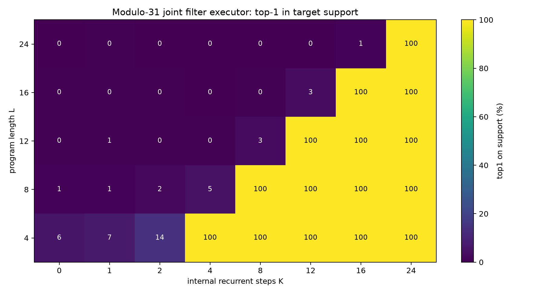
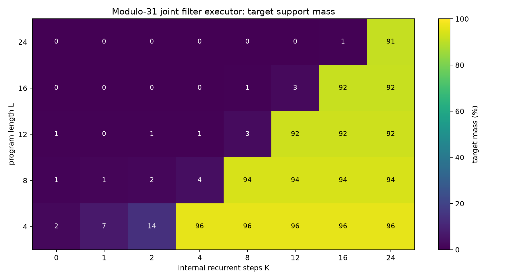
The same threshold is visible in the line curves.
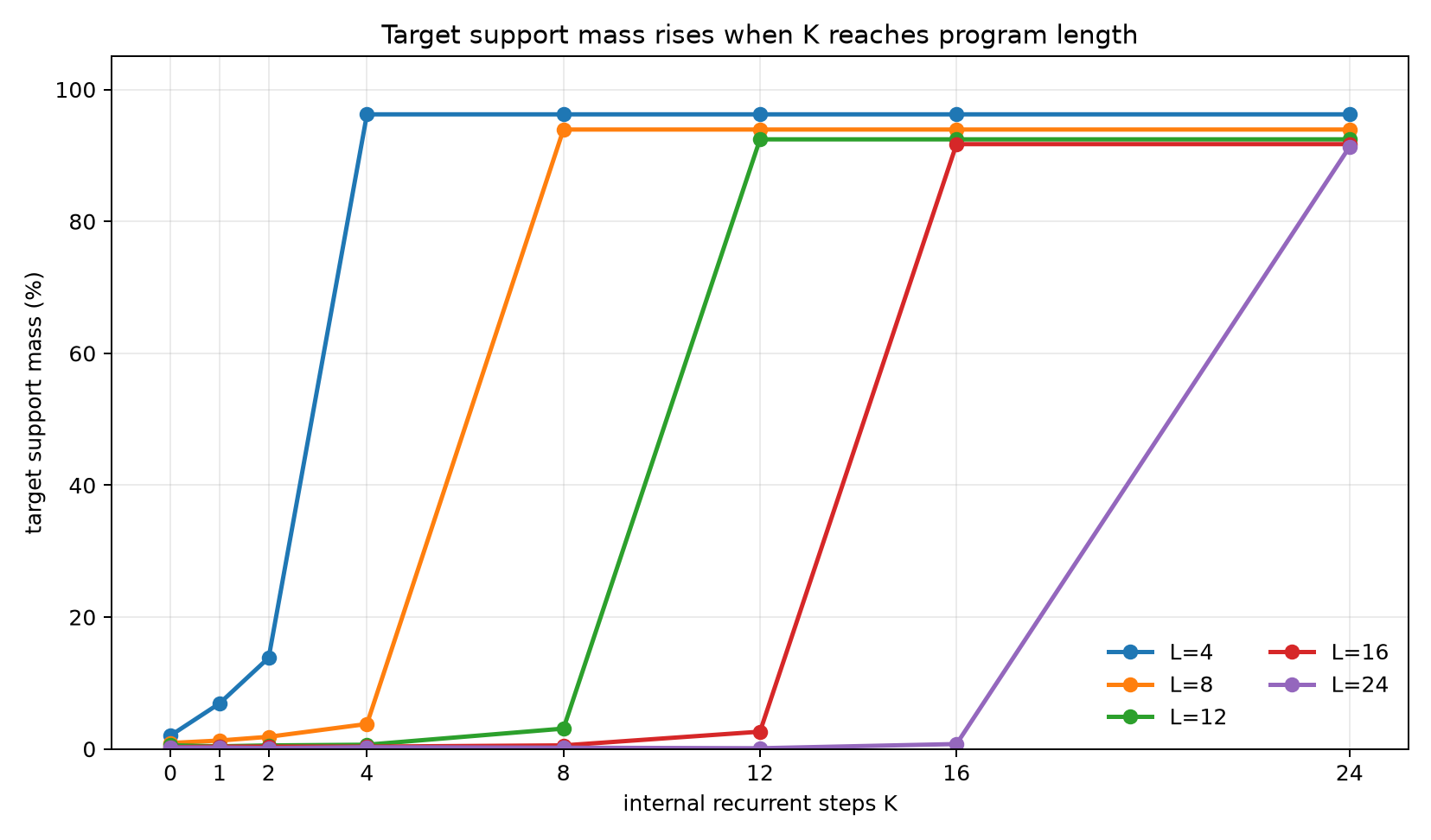
Numerically:
| Program length | Mean support size | Best target mass when K<L | First K>=L | Target mass at first K>=L | Top-1 at first K>=L | Target NLL |
|---|---|---|---|---|---|---|
| 4 | 13.1 | 13.8% | 4 | 96.2% | 100.0% | 2.195 |
| 8 | 6.5 | 3.8% | 8 | 93.9% | 100.0% | 1.500 |
| 12 | 4.2 | 3.1% | 12 | 92.4% | 100.0% | 1.081 |
| 16 | 2.7 | 2.6% | 16 | 91.7% | 100.0% | 0.785 |
| 24 | 1.7 | 0.8% | 24 | 91.3% | 100.0% | 0.441 |
The held-out lengths are the key part of the result. The model was trained only up to length 8, but it executes lengths 12, 16, and 24 when given enough recurrent steps.
6. Controls
The scaled controls show that the result is not explained by weak filtering cues or one-shot compilation.
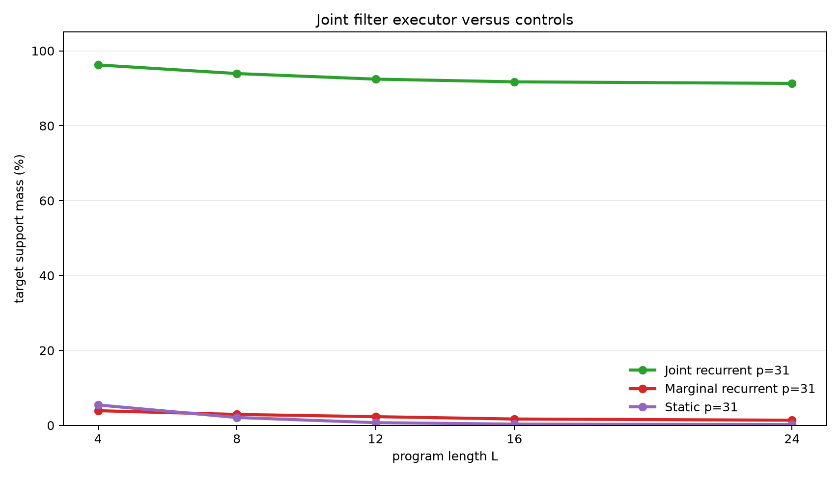
At modulus 31:
| Model | L=4 | L=8 | L=12 | L=16 | L=24 |
|---|---|---|---|---|---|
| Joint recurrent filter | 96.2% | 93.9% | 92.4% | 91.7% | 91.3% |
| Marginal recurrent control | 3.9% | 2.9% | 2.3% | 1.7% | 1.4% |
| Static compiler control | 5.4% | 2.1% | 0.7% | 0.3% | 0.2% |
The marginal control has recurrent steps and learned filters, but it cannot represent the pairwise correlation. The static compiler sees the whole program but lacks an execution axis. Both controls remain far below the joint recurrent filter on every scaled length.
7. Small-Modulus Check
A smaller modulus-11 run used the same task structure with m=4, training lengths 1-6, and evaluation lengths 3, 6, 9, and 12. The joint recurrent filter reached 92.2-96.2% target mass at the matching K=L thresholds. The matched marginal and static controls stayed below 17.5% target mass. This check established that the filtering task and controls behave consistently at a smaller state size before the modulus-31 run.
8. Interpretation
The result supports a narrow mechanism claim:
A recurrent latent runtime with a joint belief state can execute arithmetic and observation-filter programs, and additional internal steps improve performance when those steps correspond to consuming more program instructions.
The threshold shape is important:
K < L: the runtime has not executed the whole program -> low target mass
K >= L: the runtime has executed the program -> high target mass
The observations make the task stricter than pure arithmetic support transport. The model must both move probability through register updates and renormalize after filtering. The marginal control confirms that this is not solvable by tracking independent register distributions.
9. Limits
This is a structured experiment.
- The joint model stores an explicit categorical distribution over
(A,B). - Training uses dense belief supervision at program prefixes.
- The recurrent runtime uses a direct program counter.
- The operations are modular arithmetic updates and bucket observations.
- The largest completed state space has 961 pairs.
These limits define the scope of the result. The experiment shows that the mechanism works when the hidden representation is aligned with the required state. It does not show that an unstructured hidden vector will discover the same representation without additional pressure.
10. Next Iterations
Useful next tests:
- Replace the explicit program counter with attention over instruction tokens.
- Add a learned halt or no-op policy so the runtime can choose its compute budget.
- Distill the categorical belief into a dense hidden state and measure how much accuracy survives.
- Increase modulus and observation variety while tracking memory and runtime cost.
- Train on final-query supervision instead of full prefix distributions.
11. Reproducibility
Primary files:
- Experiment script:
../src/belief_filter_executor_experiment.py - Analysis script:
../src/analyze_belief_filter_executor.py - Experiment log:
belief_filter_executor_experiment_log.md - Results directory:
../runs/ - Analysis directory:
../analysis/ - Checkpoint manifest:
../checkpoint_manifest.csv
Key run directories:
../runs/main_joint_mod31../runs/control_marginal_mod31../runs/control_static_mod31../runs/pilot_joint_mod11../runs/control_marginal_mod11../runs/control_static_mod11
Large checkpoint files are stored outside the experiment bundle under:
../../../large_artifacts/belief_filter_executor/checkpoints/Environment:
- Python 3.12.3
- PyTorch 2.8.0+cu128
- GPU: NVIDIA RTX 6000 Ada Generation
12. Bottom Line
The joint recurrent filter learned to execute correlated belief-state programs with arithmetic updates and observations. It generalized from training lengths 1-8 to evaluation lengths 12, 16, and 24, and it showed a sharp improvement when the recurrent step budget reached program length. The controls failed on the same scaled task. The main lesson is that recurrent latent execution can scale cleanly with internal compute when the hidden state can represent the correlations required by the task.
Experiment log 15
Show the running log (15 entries)
Objective
Test whether a latent recurrent runtime can maintain, transform, and condition a correlated belief state over two modular registers.
The hidden state is a distribution over (A, B) pairs. Programs contain arithmetic updates and observation/filter instructions. The experiment measures whether additional recurrent steps improve exact belief-state tracking when the step budget K reaches program length L.
Hypothesis
If the runtime has a usable joint belief state, then:
- It should learn arithmetic transitions and observation filters from dense belief supervision.
- Target-support mass should be low when
K < Land high whenK >= L. - The threshold should generalize to held-out program lengths longer than training.
- A marginal recurrent control should fail because it cannot represent correlations between
AandB. - A static compiler should not reproduce the same length-generalizing K threshold.
Task
Initial belief:
B = A + d (mod p), with A unknownPrograms use:
- arithmetic operations over
AandB - observation filters of the form
A % m = r - observation filters of the form
B % m = r
Observation residues are sampled from the current support so the target support is never empty.
Models
Joint Filter Executor
The primary model stores a categorical distribution over all (A,B) pairs. At each recurrent step, it applies the next learned arithmetic transition or learned observation likelihood, then normalizes the belief state.
Marginal Filter Control
The marginal control stores separate distributions over A and B. It can condition each marginal but cannot preserve pairwise correlations.
Static Compiler Control
The static control receives the initial relation and whole program, then predicts the final belief support in one shot.
Planned Sequence
- Smoke test at tiny modulus.
- Pilot joint filter executor at small modulus.
- Matched marginal and static controls at small modulus.
- Main scaled run at modulus 31.
- Matched scaled controls.
- Aggregate metrics, generate figures, and write a standalone report.
Smoke Test
Run: ../runs/smoke_joint_mod7
Configuration:
- mode: joint
- modulus: 7
- observation modulus: 3
- observation probability: 0.4
- train length max: 3
- train steps: 2
- eval lengths: 2, 3
Result: the script compiled, trained, evaluated, wrote metrics, and saved checkpoints under ../../../large_artifacts/belief_filter_executor/checkpoints/smoke_joint_mod7.
Interpretation: arithmetic transitions, observation filters, belief targets, evaluation metrics, and separated checkpoint writing are functional. The run is intentionally too short to test learning.
Pilot 1: Joint Filter Executor, Modulus 11
Run: ../runs/pilot_joint_mod11
Configuration:
- mode: joint
- modulus: 11
- observation modulus: 4
- observation probability: 0.3
- train lengths: 1-6
- eval lengths: 3, 6, 9, 12
- recurrent budgets:
K=0,1,2,3,6,9,12 - eval examples: 1,024 per length
- training steps: 300
Result at step 300:
L=3:K=3reached 100% top-1-on-support and 96.2% target mass.L=6:K=6reached 100% top-1-on-support and 94.1% target mass.L=9:K=9reached 100% top-1-on-support and 93.0% target mass.L=12:K=12reached 100% top-1-on-support and 92.2% target mass.
For K<L, target mass stayed far below the sufficient-K values. This is the first positive result that the joint runtime can combine arithmetic transitions and observation filters.
Control 1: Marginal Filter Executor, Modulus 11
Run: ../runs/control_marginal_mod11
Configuration matched Pilot 1 except mode=marginal.
Result at step 300:
L=3: best sufficient-K target mass 10.7%.L=6: best sufficient-K target mass 10.2%.L=9: best sufficient-K target mass 8.9%.L=12: best sufficient-K target mass 7.9%.
Interpretation: the marginal model can learn some filtering behavior, but it cannot reconstruct the joint support. It remains far below the joint executor's 92-96% target mass.
Control 2: Static Filter Compiler, Modulus 11
Run: ../runs/control_static_mod11
Configuration matched Pilot 1 except mode=static.
Result at step 300:
L=3: 17.5% target mass.L=6: 8.2% target mass.L=9: 3.4% target mass.L=12: 2.3% target mass.
Interpretation: the static compiler learns some short-length signal but does not solve longer held-out programs.
Main Run: Joint Filter Executor, Modulus 31
Run: ../runs/main_joint_mod31
Configuration:
- mode: joint
- modulus: 31
- observation modulus: 5
- observation probability: 0.3
- train lengths: 1-8
- eval lengths: 4, 8, 12, 16, 24
- recurrent budgets:
K=0,1,2,4,8,12,16,24 - eval examples: 1,024 per length
- training steps: 500
Result at step 500:
L=4:K=4reached 100% top-1-on-support and 96.2% target mass.L=8:K=8reached 100% top-1-on-support and 93.9% target mass.L=12:K=12reached 100% top-1-on-support and 92.4% target mass.L=16:K=16reached 100% top-1-on-support and 91.7% target mass.L=24:K=24reached 100% top-1-on-support and 91.3% target mass.
For K<L, target mass stayed near zero on long programs, with only partial-prefix gains. This is the main positive result.
Scaled Control: Marginal Filter Executor, Modulus 31
Run: ../runs/control_marginal_mod31
Configuration matched the main run except mode=marginal and 300 training steps.
Result at step 300:
L=4: best sufficient-K target mass 3.9%.L=8: best sufficient-K target mass 2.9%.L=12: best sufficient-K target mass 2.3%.L=16: best sufficient-K target mass 1.7%.L=24: best sufficient-K target mass 1.4%.
Interpretation: the marginal model learns weak filtering signals but cannot preserve the joint support.
Scaled Control: Static Filter Compiler, Modulus 31
Run: ../runs/control_static_mod31
Configuration matched the main run except mode=static and 300 training steps.
Result at step 300:
L=4: 5.4% target mass.L=8: 2.1% target mass.L=12: 0.7% target mass.L=16: 0.3% target mass.L=24: 0.2% target mass.
Interpretation: the static compiler does not solve the scaled filtered belief task and does not length-generalize.
Figures 4
Data files 22
Result tables and metrics copied from the experiment folder — preview inline or open the raw file.
analysis/all_metrics_long.csv31 kBanalysis/final_metrics_long.csv19 kBanalysis/mod31_control_summary.csv1.3 kBanalysis/mod31_threshold_summary.csv536 Bruns/control_marginal_mod11/metrics_step00300.csv2.3 kBruns/control_marginal_mod11/results.json11 kBruns/control_marginal_mod31/metrics_step00300.csv3.4 kBruns/control_marginal_mod31/results.json15 kBruns/control_static_mod11/metrics_step00300.csv392 Bruns/control_static_mod11/results.json4.1 kBruns/control_static_mod31/metrics_step00300.csv486 Bruns/control_static_mod31/results.json4.4 kBruns/main_joint_mod31/metrics_step00250.csv3.1 kBruns/main_joint_mod31/metrics_step00500.csv3.2 kBruns/main_joint_mod31/results.json30 kBruns/pilot_joint_mod11/metrics_step00100.csv2.1 kBruns/pilot_joint_mod11/metrics_step00200.csv2.2 kBruns/pilot_joint_mod11/metrics_step00300.csv2.2 kBruns/pilot_joint_mod11/results.json29 kBruns/smoke_joint_mod7/metrics_step00001.csv600 Bruns/smoke_joint_mod7/metrics_step00002.csv609 Bruns/smoke_joint_mod7/results.json6.2 kB
Reproduce
The run commands are documented inside the experiment folder (see the README).